Concurrent Validity
a04_Vignette_Concurrent_Validity.RmdIllustration of Concurrent Validity
Here we are using the polycor R package to compute the correlations. The COA34 functions are just wrappers for that R package functions that prepare the output. I think the scatter plot of the correlations was well-received, worth including that.
Generate data
  set.seed(12162021)

  sim.out <- COA34::sim_pro_dat_v2(N=1000,
                            number.timepoints = 3,
                            Beta.PRO = NULL,
                            number.of.anchor.groups = 5,
                            polychor.value = 0.7,
                            corr = 'ar1',
                            cor.value = 0.8,
                            #var.values = c(7.136))
                            var.values = c(2))
  dat <- sim.out$dat
Simulate Items
 # Simulate IRT items
 # use the scores generated as the theta in the IRT model
  sim.out2 <- COA34::sim_irt_item(dat = dat, J = 5, K = 4, latent.variable = 'Y_comp')
    str(sim.out2)
#> List of 3
#>  $ dat           :'data.frame':  3000 obs. of  22 variables:
#>   ..$ USUBJID   : chr [1:3000] "Subject_0001" "Subject_0001" "Subject_0001" "Subject_0002" ...
#>   ..$ Time      : Factor w/ 3 levels "Time_1","Time_2",..: 1 2 3 1 2 3 1 2 3 1 ...
#>   ..$ PGIS      : num [1:3000] 3 4 3 0 0 0 0 0 1 1 ...
#>   ..$ PGIS_bl   : num [1:3000] 3 3 3 0 0 0 0 0 0 1 ...
#>   ..$ PGIS_delta: num [1:3000] 0 1 0 0 0 0 0 0 1 0 ...
#>   ..$ ag        : num [1:3000] 0 1 0 0 0 0 0 0 1 0 ...
#>   ..$ XB        : num [1:3000] 4 4.25 4 1 1 1 1 1 2 2 ...
#>   ..$ error     : num [1:3000] -0.336 -0.509 0.122 0.825 1.212 ...
#>   ..$ Y_comp    : num [1:3000] 3.66 3.74 4.12 1.82 2.21 ...
#>   ..$ Val_1     : int [1:3000] 2 NA NA 0 NA NA 0 NA NA 0 ...
#>   ..$ Val_2     : num [1:3000] 6.38 NA NA 3.87 NA ...
#>   ..$ Val_3     : num [1:3000] 3.73 NA NA 4.57 NA ...
#>   ..$ Val_4     : num [1:3000] 0.555 NA NA 1.558 NA ...
#>   ..$ Val_5     : int [1:3000] 4 NA NA 4 NA NA 0 NA NA 2 ...
#>   ..$ Y_mcar    : num [1:3000] 3.66 3.74 NA 1.82 2.21 ...
#>   ..$ Y_mar     : num [1:3000] 3.66 3.74 NA 1.82 2.21 ...
#>   ..$ Y_mnar    : num [1:3000] 3.66 3.74 NA 1.82 2.21 ...
#>   ..$ Item_1    : int [1:3000] 2 2 2 1 1 1 0 1 0 1 ...
#>   ..$ Item_2    : int [1:3000] 3 1 3 0 2 3 0 0 0 0 ...
#>   ..$ Item_3    : int [1:3000] 2 2 2 1 1 3 0 0 0 0 ...
#>   ..$ Item_4    : int [1:3000] 3 3 1 0 0 2 2 0 1 0 ...
#>   ..$ Item_5    : int [1:3000] 2 2 2 1 0 1 0 0 1 1 ...
#>  $ item.param    : num [1:5, 1:4] 2 2 2 2 2 -2 -2 -2 -2 -2 ...
#>   ..- attr(*, "dimnames")=List of 2
#>   .. ..$ : chr [1:5] "Item_1" "Item_2" "Item_3" "Item_4" ...
#>   .. ..$ : chr [1:4] "slope" "intercept_1" "intercept_2" "intercept_3"
#>  $ item.responses:'data.frame':  3000 obs. of  5 variables:
#>   ..$ Item_1: int [1:3000] 2 2 2 1 1 1 0 1 0 1 ...
#>   ..$ Item_2: int [1:3000] 3 1 3 0 2 3 0 0 0 0 ...
#>   ..$ Item_3: int [1:3000] 2 2 2 1 1 3 0 0 0 0 ...
#>   ..$ Item_4: int [1:3000] 3 3 1 0 0 2 2 0 1 0 ...
#>   ..$ Item_5: int [1:3000] 2 2 2 1 0 1 0 0 1 1 ...
    dat <- sim.out2$dat

# Score the PRO - just take a simple sum score here:
  dat$PRO.score <- apply(dat[, grep('Item', colnames(dat))], 1, sum)

# Create the same PRO score, but with MAR drop-out:
  dat$PRO.score_mar <- dat$PRO.score
  dat$PRO.score_mar[is.na(dat$Y_mar)] <- NA
# Note that you've just set the PRO score to missing wherever the Y_mar variable is missing

# Now for the other missing types:
    dat$PRO.score_mcar <- dat$PRO.score_mnar <- dat$PRO.score
    dat$PRO.score_mcar[is.na(dat$Y_mcar)] <- NA
    dat$PRO.score_mnar[is.na(dat$Y_mnar)] <- NA

  aggregate(cbind(PRO.score, PRO.score_mcar, PRO.score_mar, PRO.score_mnar) ~ Time,
                  function(x) mean(x, na.rm = T),
                  data = dat,
                  na.action = na.pass)
#>     Time PRO.score PRO.score_mcar PRO.score_mar PRO.score_mnar
#> 1 Time_1     7.445       7.445000         7.445          7.445
#> 2 Time_2     7.492       7.486667         5.912          5.748
#> 3 Time_3     7.520       7.736000         5.210          4.204
Managing Variables
I can’t overemphasize how important it is to keep an eye on your variables. The functions will do all the work, you just have to carefully manage your data.
str(dat)
#> 'data.frame':    3000 obs. of  26 variables:
#>  $ USUBJID       : chr  "Subject_0001" "Subject_0001" "Subject_0001" "Subject_0002" ...
#>  $ Time          : Factor w/ 3 levels "Time_1","Time_2",..: 1 2 3 1 2 3 1 2 3 1 ...
#>  $ PGIS          : num  3 4 3 0 0 0 0 0 1 1 ...
#>  $ PGIS_bl       : num  3 3 3 0 0 0 0 0 0 1 ...
#>  $ PGIS_delta    : num  0 1 0 0 0 0 0 0 1 0 ...
#>  $ ag            : num  0 1 0 0 0 0 0 0 1 0 ...
#>  $ XB            : num  4 4.25 4 1 1 1 1 1 2 2 ...
#>  $ error         : num  -0.336 -0.509 0.122 0.825 1.212 ...
#>  $ Y_comp        : num  3.66 3.74 4.12 1.82 2.21 ...
#>  $ Val_1         : int  2 NA NA 0 NA NA 0 NA NA 0 ...
#>  $ Val_2         : num  6.38 NA NA 3.87 NA ...
#>  $ Val_3         : num  3.73 NA NA 4.57 NA ...
#>  $ Val_4         : num  0.555 NA NA 1.558 NA ...
#>  $ Val_5         : int  4 NA NA 4 NA NA 0 NA NA 2 ...
#>  $ Y_mcar        : num  3.66 3.74 NA 1.82 2.21 ...
#>  $ Y_mar         : num  3.66 3.74 NA 1.82 2.21 ...
#>  $ Y_mnar        : num  3.66 3.74 NA 1.82 2.21 ...
#>  $ Item_1        : int  2 2 2 1 1 1 0 1 0 1 ...
#>  $ Item_2        : int  3 1 3 0 2 3 0 0 0 0 ...
#>  $ Item_3        : int  2 2 2 1 1 3 0 0 0 0 ...
#>  $ Item_4        : int  3 3 1 0 0 2 2 0 1 0 ...
#>  $ Item_5        : int  2 2 2 1 0 1 0 0 1 1 ...
#>  $ PRO.score     : int  12 10 10 3 4 10 2 1 2 2 ...
#>  $ PRO.score_mar : int  12 10 NA 3 4 10 2 1 2 2 ...
#>  $ PRO.score_mnar: int  12 10 NA 3 4 10 2 1 2 2 ...
#>  $ PRO.score_mcar: int  12 10 NA 3 4 10 2 1 NA 2 ...
# PGIS is ordinal; transform it for the purposes of correct correlation
# Leave it numeric to compute the PGIS_delta for the change scores later
dat.cor <- dat
dat.cor$PGIS <-
  factor(dat.cor$PGIS,
         levels = c(0, 1, 2, 3, 4),
         labels = c('None', 'Mild', 'Moderate', 'Severe', 'Very Severe'))
table(dat.cor$PGIS, useNA = 'always')
#>
#>        None        Mild    Moderate      Severe Very Severe        <NA>
#>         683         604         621         526         566           0
xtabs(~ dat.cor$PGIS + dat$PGIS)
#>              dat$PGIS
#> dat.cor$PGIS    0   1   2   3   4
#>   None        683   0   0   0   0
#>   Mild          0 604   0   0   0
#>   Moderate      0   0 621   0   0
#>   Severe        0   0   0 526   0
#>   Very Severe   0   0   0   0 566

# Validator Variables 1 and 5 are supposed to be
# ordered categorical variables
dat.cor$Val_1 <- factor(dat.cor$Val_1)
table(dat.cor$Val_1, useNA = 'always')
#>
#>    0    1    2 <NA>
#>  334  333  333 2000
# only collected at baseline, hence the NAs

dat.cor$Val_5 <- factor(dat.cor$Val_5)
table(dat.cor$Val_5, useNA = 'always')
#>
#>    0    1    2    3    4 <NA>
#>  200  200  200  200  200 2000
# Only collected at baseline, hence the NAs

# Check data:
str(dat.cor)
#> 'data.frame':    3000 obs. of  26 variables:
#>  $ USUBJID       : chr  "Subject_0001" "Subject_0001" "Subject_0001" "Subject_0002" ...
#>  $ Time          : Factor w/ 3 levels "Time_1","Time_2",..: 1 2 3 1 2 3 1 2 3 1 ...
#>  $ PGIS          : Factor w/ 5 levels "None","Mild",..: 4 5 4 1 1 1 1 1 2 2 ...
#>  $ PGIS_bl       : num  3 3 3 0 0 0 0 0 0 1 ...
#>  $ PGIS_delta    : num  0 1 0 0 0 0 0 0 1 0 ...
#>  $ ag            : num  0 1 0 0 0 0 0 0 1 0 ...
#>  $ XB            : num  4 4.25 4 1 1 1 1 1 2 2 ...
#>  $ error         : num  -0.336 -0.509 0.122 0.825 1.212 ...
#>  $ Y_comp        : num  3.66 3.74 4.12 1.82 2.21 ...
#>  $ Val_1         : Factor w/ 3 levels "0","1","2": 3 NA NA 1 NA NA 1 NA NA 1 ...
#>  $ Val_2         : num  6.38 NA NA 3.87 NA ...
#>  $ Val_3         : num  3.73 NA NA 4.57 NA ...
#>  $ Val_4         : num  0.555 NA NA 1.558 NA ...
#>  $ Val_5         : Factor w/ 5 levels "0","1","2","3",..: 5 NA NA 5 NA NA 1 NA NA 3 ...
#>  $ Y_mcar        : num  3.66 3.74 NA 1.82 2.21 ...
#>  $ Y_mar         : num  3.66 3.74 NA 1.82 2.21 ...
#>  $ Y_mnar        : num  3.66 3.74 NA 1.82 2.21 ...
#>  $ Item_1        : int  2 2 2 1 1 1 0 1 0 1 ...
#>  $ Item_2        : int  3 1 3 0 2 3 0 0 0 0 ...
#>  $ Item_3        : int  2 2 2 1 1 3 0 0 0 0 ...
#>  $ Item_4        : int  3 3 1 0 0 2 2 0 1 0 ...
#>  $ Item_5        : int  2 2 2 1 0 1 0 0 1 1 ...
#>  $ PRO.score     : int  12 10 10 3 4 10 2 1 2 2 ...
#>  $ PRO.score_mar : int  12 10 NA 3 4 10 2 1 2 2 ...
#>  $ PRO.score_mnar: int  12 10 NA 3 4 10 2 1 2 2 ...
#>  $ PRO.score_mcar: int  12 10 NA 3 4 10 2 1 NA 2 ...
# 5 validator variables (Val_1, Val_2...Val_5)
# 4 PRO scores
Compute Correlations of Multiple Scores
Use the function to create a large table of the correlations you need.
Note that the correlations are computed using baseline data, with no missingness. Thus, all of the different types of drop-out will have the exact same values. This table is, of course, just to illustrate the functionality.
If this isn’t exactly what you’re looking for, try the hetcor() function in the polycor R package.
out <- COA34::compute_validity(dat = dat.cor,
                               time.var = 'Time',
                               PRO.score = c('PRO.score',
                                             'PRO.score_mcar',
                                             'PRO.score_mar',
                                             'PRO.score_mnar'),
                               val.var = c('PGIS', paste0('Val_', 1:5))
                               )

# Compare output to generating values:
sim.out$out.val$cor.mat.ref
#>       Score Val_1 Val_2 Val_3 Val_4 Val_5
#> Score   1.0  0.50  0.60  0.80  0.20  0.30
#> Val_1   0.5  1.00  0.30  0.40  0.10  0.15
#> Val_2   0.6  0.30  1.00  0.48  0.12  0.18
#> Val_3   0.8  0.40  0.48  1.00  0.16  0.24
#> Val_4   0.2  0.10  0.12  0.16  1.00  0.06
#> Val_5   0.3  0.15  0.18  0.24  0.06  1.00

library(R2Word)

R2Word::dump_df_mat_to_file(out = out,
                            decimals = c(0, 2),
                            table.title = 'Correlations - Vignette Illustration',
                            table.footnote = '**All data simulated',
                            file.name = 'val_vig_t1',
print.dir = print.dir)Correlations - Vignette Illustration | ||||
PRO Score |
Validator Variable |
Correlation Type |
Sample Size |
Correlation |
PRO.score |
PGIS |
polyserial |
1000 |
0.81 |
PRO.score |
Val_1 |
polyserial |
1000 |
0.52 |
PRO.score |
Val_2 |
Pearson |
1000 |
0.55 |
PRO.score |
Val_3 |
Pearson |
1000 |
0.73 |
PRO.score |
Val_4 |
Pearson |
1000 |
0.19 |
PRO.score |
Val_5 |
polyserial |
1000 |
0.30 |
PRO.score_mcar |
PGIS |
polyserial |
1000 |
0.81 |
PRO.score_mcar |
Val_1 |
polyserial |
1000 |
0.52 |
PRO.score_mcar |
Val_2 |
Pearson |
1000 |
0.55 |
PRO.score_mcar |
Val_3 |
Pearson |
1000 |
0.73 |
PRO.score_mcar |
Val_4 |
Pearson |
1000 |
0.19 |
PRO.score_mcar |
Val_5 |
polyserial |
1000 |
0.30 |
PRO.score_mar |
PGIS |
polyserial |
1000 |
0.81 |
PRO.score_mar |
Val_1 |
polyserial |
1000 |
0.52 |
PRO.score_mar |
Val_2 |
Pearson |
1000 |
0.55 |
PRO.score_mar |
Val_3 |
Pearson |
1000 |
0.73 |
PRO.score_mar |
Val_4 |
Pearson |
1000 |
0.19 |
PRO.score_mar |
Val_5 |
polyserial |
1000 |
0.30 |
PRO.score_mnar |
PGIS |
polyserial |
1000 |
0.81 |
PRO.score_mnar |
Val_1 |
polyserial |
1000 |
0.52 |
PRO.score_mnar |
Val_2 |
Pearson |
1000 |
0.55 |
PRO.score_mnar |
Val_3 |
Pearson |
1000 |
0.73 |
PRO.score_mnar |
Val_4 |
Pearson |
1000 |
0.19 |
PRO.score_mnar |
Val_5 |
polyserial |
1000 |
0.30 |
**All data simulated | ||||
Scatterplots of Correlations
Let’s compute for a single score and create a scatterplot. This visualization has been well-received, make use of it.
out1 <- COA34::compute_validity(dat = dat.cor,
                               time.var = 'Time',
                               PRO.score = 'PRO.score',
                               val.var = c('PGIS', paste0('Val_', 1:5))
                               )
We have the output values, let’s make the scatterplot:
# Scatterplot of Correlations:
library(ggplot2)
p1 <- ggplot(out1, aes(x = `Validator Variable`, y = Correlation)) +
  geom_point() +
  theme_minimal() +
  theme(axis.text.x=element_blank()) +
  scale_y_continuous(lim = c(0,1), breaks = seq(0, 1, by = 0.1))

library(ggrepel)
p2 <- p1 + ggrepel::geom_text_repel(aes(label = `Validator Variable`),
              size = 3.5)
p2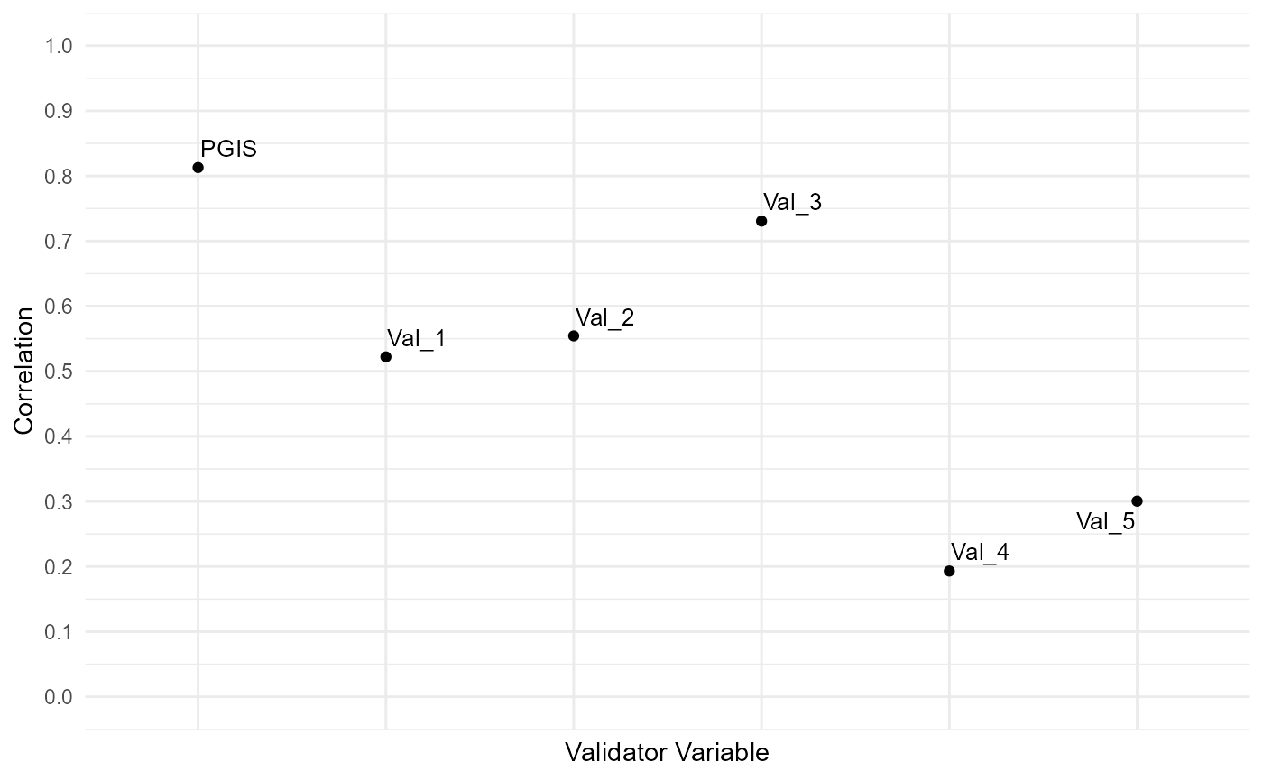
# How to customize the labels
out1$label <-
  ifelse(out1$`Validator Variable` == 'PGIS', 'PGIS anchor',
         ifelse(out1$`Validator Variable` == 'Val_1', 'PGIC',
                ifelse(out1$`Validator Variable` == 'Val_2', 'SF-36',
                       ifelse(out1$`Validator Variable` == 'Val_3', 'EQ-5D',
                              ifelse(out1$`Validator Variable` == 'Val_4', 'NSCLC-SAQ',
                                     ifelse(out1$`Validator Variable` == 'Val_5', 'SF-36, Physical Functioning',
                                            NA))))))

library(ggrepel)
p3 <- p1 + ggrepel::geom_text_repel(data = out1, aes(label = `label`),
              size = 3.5)
p3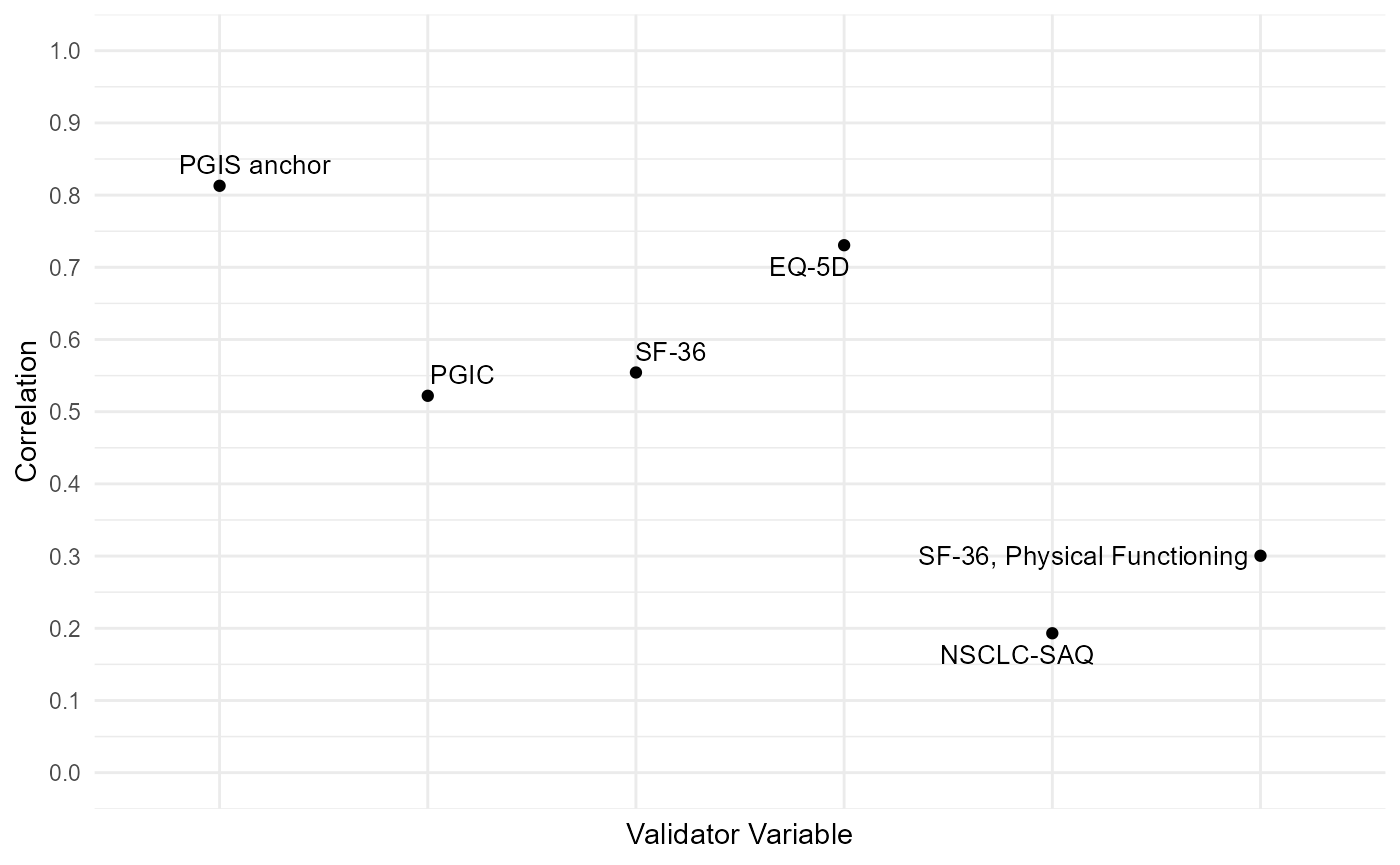
Note on timepoints
The compute_validity() function will automatically select the baseline timepoint. If you want to use a different timepoint, you’ll have to pass a dataframe with only that data! Quick example:
out2 <- COA34::compute_validity(dat = dat.cor[dat.cor$Time == 'Time_3', ],
                               time.var = 'Time',
                               PRO.score = c('PRO.score',
                                             'PRO.score_mcar',
                                             'PRO.score_mar',
                                             'PRO.score_mnar'),
                               val.var = c('PGIS'))

out2
#>        PRO Score Validator Variable Correlation Type Sample Size Correlation
#> 1      PRO.score               PGIS       polyserial        1000   0.6555130
#> 2 PRO.score_mcar               PGIS       polyserial         500   0.6473966
#> 3  PRO.score_mar               PGIS       polyserial         500   0.5888753
#> 4 PRO.score_mnar               PGIS       polyserial         500   0.3349494