Continuous Data (Normal error distribution)

Review and run the code below to better understand the data distribution.

1. TODO: Add a simulation study code
2. TODO: pull the hessian and estimate SE

Generate cross sectional data

library(SPR)
library(MASS)


N = 1000 #this should be divisible by however many groups you use!
number.groups <- 2
number.timepoints <- 1
#set.seed(2182021)

    dat <- data.frame(
                      'USUBJID' = rep(paste0('Subject_', formatC(1:N, width = 4, flag = '0')), length.out= N*number.timepoints),
                      'Group' = rep(paste0('Group_', 1:number.groups), length.out = N*number.timepoints),
                      'Y_comp' = rep(NA, N*number.timepoints), 
                      #'Bio' = rep(rnorm(N, mean = 0, sd = 1), number.timepoints),
                      'Time' = rep(paste0('Time_', 1:number.timepoints), each = N),
                      stringsAsFactors=F)
    
        
        # Design Matrix
    X <- model.matrix( ~ Group , data = dat) 
    Beta <- matrix(0, nrow = ncol(X), dimnames=list(colnames(X), 'param'))
    Beta[] <- c(0.2, 1)
    sigma2 <- 9 
    
    # Parameters:
    XB <- X %*% Beta
    dat$XB <- as.vector(XB)
    error <- rnorm(n = N, mean = 0, sd = sqrt(sigma2))
    dat$Y <- dat$XB + error

Plot

    # check
    hist(dat$Y)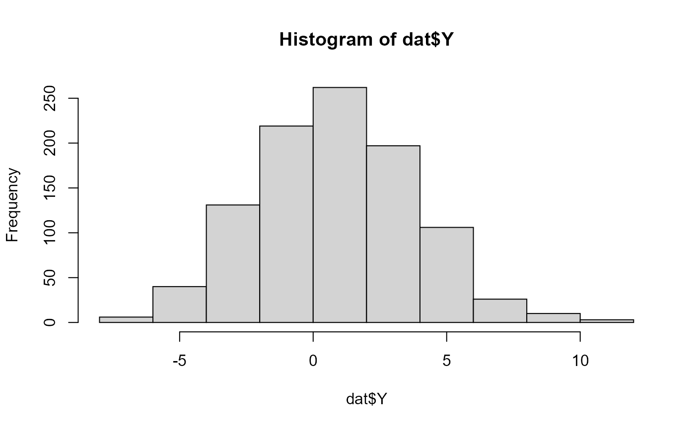

    aggregate(Y ~ 1, FUN = mean, data = dat)
#>           Y
#> 1 0.8448831
    aggregate(Y ~ Group, FUN = mean, data = dat)
#>     Group         Y
#> 1 Group_1 0.2998085
#> 2 Group_2 1.3899577
    aggregate(Y ~ Group, FUN = var, data = dat)
#>     Group        Y
#> 1 Group_1 8.282694
#> 2 Group_2 9.151022
    
    # Model?
    mod <-lm(Y ~ Group, data = dat)
    summary(mod)
#> 
#> Call:
#> lm(formula = Y ~ Group, data = dat)
#> 
#> Residuals:
#>     Min      1Q  Median      3Q     Max 
#> -8.2425 -2.0412 -0.0239  1.9320 10.3740 
#> 
#> Coefficients:
#>              Estimate Std. Error t value Pr(>|t|)    
#> (Intercept)    0.2998     0.1320   2.271   0.0234 *  
#> GroupGroup_2   1.0901     0.1867   5.838 7.13e-09 ***
#> ---
#> Signif. codes:  0 '***' 0.001 '**' 0.01 '*' 0.05 '.' 0.1 ' ' 1
#> 
#> Residual standard error: 2.952 on 998 degrees of freedom
#> Multiple R-squared:  0.03302,    Adjusted R-squared:  0.03206 
#> F-statistic: 34.08 on 1 and 998 DF,  p-value: 7.133e-09
    summary(mod)$sigma
#> [1] 2.952433
    # g2g
  

Run custom estimation code

This is helpful because it shows you the likelihood

vP <- c('b0' = 0.2, 'b1' = 1)

Normal_loglike <- function(vP, dat){
  
  Beta.hat <- vP[c('b0', 'b1')]
  Beta.hat <- matrix(Beta.hat, ncol = 1)
  X <- model.matrix( ~ Group , data = dat) 
  Y.hat <- X %*% Beta.hat 
  SSE <- sum((Y.hat - dat$Y)^2)
  return(SSE)

}



# optimize
vP <- c('b0' = 0.2, 'b1' = 1)
out <- optim(par = vP, fn = Normal_loglike, method = 'BFGS', dat = dat)

# Use Beta.hat to estimate the sigma:
Beta.hat <- out$par
Beta.hat <- matrix(Beta.hat, ncol = 1)
X <- model.matrix( ~ Group , data = dat) 
Y.hat <- X %*% Beta.hat 
sigma2.hat <- sum((Y.hat - dat$Y)^2)/(N-2)  # N-p-1, where p is number of predictors

# Compare observed vs predicted:
mean(Y.hat)
#> [1] 0.8448832
mean(dat$Y)
#> [1] 0.8448831
# Compare parameter estimates:
cbind(
  'Gen param' = c(Beta, sigma2), 
  'Custom Function' = c(out$par, sigma2.hat), 
  'R package' = c(coef(mod), summary(mod)$sigma^2)
)
#>    Gen param Custom Function R package
#> b0       0.2       0.2998086 0.2998085
#> b1       1.0       1.0901492 1.0901492
#>          9.0       8.7168581 8.7168581