Relative Risk and Odds Ratios
a07_1_Relative_Risk.RmdOdds ratios can be difficult to interpret. Relative risk is typically easier to interpret. However, computation of RR requires the base rate, or base prevalence. This tutorial will focus on
Show you what the relative risk is (note that we already reviewed the odds ratio in a previous tutorial).
Show you how to estimate the RR from a log binomial model.
Show you how to estimate the RR from a logistic regression model. This is simple when you are computing an unadjusted estimate of RR. Once you add covariates into the model, things are less simple.
Background Reading
Doi SA, Furuya-Kanamori L, Xu C, Chivese T, Lin L, Musa OA, Hindy G, Thalib L, Harrell Jr FE. The odds ratio is “portable” but not the relative risk: Time to do away with the log link in binomial regression. Journal of Clinical Epidemiology. 2021 Aug 8. https://www.sciencedirect.com/science/article/abs/pii/S0895435621002419?dgcid=coauthor
Doi SA, Furuya-Kanamori L, Xu C, Lin L, Chivese T, Thalib L. Questionable utility of the relative risk in clinical research: a call for change to practice. Journal of Clinical Epidemiology. 2020 Nov 7. https://www.sciencedirect.com/science/article/pii/S0895435620311719
Zhu and Yang, 1998: https://jamanetwork.com/journals/jama/fullarticle/188182
More details:
Marginalization over covariates: https://academic.oup.com/ije/article/43/3/962/763470?login=true
Adjustments and Collapsability: https://escholarship.org/content/qt3ng2r0sm/qt3ng2r0sm.pdf
Relative Risk Regression in Medical Research: Models, Contrasts, Estimators, and Algorithms https://core.ac.uk/download/pdf/61319711.pdf
Simulate Data
Simulate cross-sectional prevalence data. Note that we are using the log link function p <- exp(XB) instead of the logit link p <- exp(XB)/(1 + exp(XB)) The latter is logistic regression.
library(SPR)
library(MASS)

N = 1e5 #this should be divisible by however many groups you use!
number.groups <- 2
number.timepoints <- 1
set.seed(9062021)

dat <- data.frame(
                  'USUBJID' = rep(paste0('Subject_', formatC(1:N, width = 4, flag = '0')), length.out= N*number.timepoints),
                  'Group' = rep(paste0('Group_', 1:number.groups), length.out = N*number.timepoints),
                  stringsAsFactors=F)


# Create Beta parameters for these design matrix:
X <- model.matrix( ~ Group  , data = dat)

# Create Beta
Beta <- matrix(0, nrow = ncol(X), dimnames=list(colnames(X), 'param'))
Beta[] <- c(-0.5, -1)

# Matrix multiply:
XB <- X %*% Beta
p <- exp(XB) # prevalence - log link
#p <- exp(XB)/(1 + exp(XB)) - this is the logistic link
round(range(p), 2)
#> [1] 0.22 0.61

# Dichotomize
dat$Y_binom <- 1*(p > runif(n = N))

# Plot
aggregate(Y_binom  ~ Group, FUN = function(x) round(mean(x, na.rm = T),2), dat = dat, na.action = na.pass)
#>     Group param
#> 1 Group_1  0.60
#> 2 Group_2  0.22
barplot(100*table(dat$Y_binom )/sum(table(dat$Y_binom )), ylim = c(0, 100), ylab = 'Percentage', col = 'grey', main = 'Binomial')


library(ggplot2)
ggplot(data = dat, aes(x= as.factor(Y_binom), fill = Group)) +
      geom_bar(aes(y = (..count..)/sum(..count..)), color="#e9ecef", alpha=0.6, position="dodge", stat="count") +
      scale_y_continuous(labels=scales::percent_format(accuracy = 1)) +
      scale_fill_manual(name = 'Groups', values=c("blue2", "red2")) +
      theme_minimal() +
      theme(legend.position = 'bottom') +
      labs(x = 'Score', y = 'Percentage',
           title = 'Scores with a Binomial Distribution',
           caption = 'Note: Simulated data')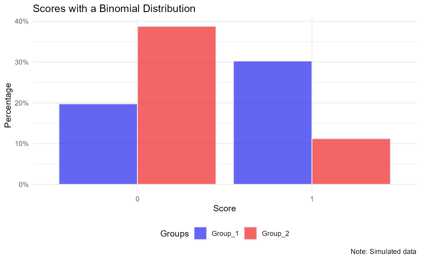
# Observed Data:
xtabs(~ Y_binom + Group, data = dat)
#>        Group
#> Y_binom Group_1 Group_2
#>       0   19756   38769
#>       1   30244   11231
ptab <- prop.table(xtabs(~ Y_binom + Group, data = dat), 2)
# Percentage achieving "1" across Groups:
ptab
#>        Group
#> Y_binom Group_1 Group_2
#>       0 0.39512 0.77538
#>       1 0.60488 0.22462
The object ptab is the table of proportions. We then fit models and compare the model output to the observed.
Model Fitting - Log Binomial Model
This models the relative risk directly. Unfortunately, it tends to be difficult to estimate and not fit the data as well as the logit link model (i.e., logistic regression).
# Compare to model output:
mod <- glm(Y_binom ~ Group, data = dat, family = binomial(link ='log'))
summary(mod)
#>
#> Call:
#> glm(formula = Y_binom ~ Group, family = binomial(link = "log"),
#>     data = dat)
#>
#> Deviance Residuals:
#>     Min       1Q   Median       3Q      Max
#> -1.3628  -0.7133  -0.7133   1.0027   1.7282
#>
#> Coefficients:
#>               Estimate Std. Error z value Pr(>|z|)
#> (Intercept)  -0.502725   0.003614  -139.1   <2e-16 ***
#> GroupGroup_2 -0.990620   0.009061  -109.3   <2e-16 ***
#> ---
#> Signif. codes:  0 '***' 0.001 '**' 0.01 '*' 0.05 '.' 0.1 ' ' 1
#>
#> (Dispersion parameter for binomial family taken to be 1)
#>
#>     Null deviance: 135708  on 99999  degrees of freedom
#> Residual deviance: 120368  on 99998  degrees of freedom
#> AIC: 120372
#>
#> Number of Fisher Scoring iterations: 6
exp(coef(mod)['(Intercept)' ]) # Group 1
#> (Intercept)
#>     0.60488
exp(sum(coef(mod))) # Group 2
#> [1] 0.22462
# equal to observed - won't be equal if adjusted (i.e., other variables in model)


# Observed Data: What is the relative risk?
ptab['1', 'Group_2']/ptab['1', 'Group_1']
#> [1] 0.3713464
# Group 1 is almost 3 times as likely to have event as Group 2

# model estimate of relative risk:
exp(coef(mod)['GroupGroup_2'])
#> GroupGroup_2
#>    0.3713464
# aligned with observed - remember this only lines up exactly because
# you have no other variables in the model. If you include other variables,
# then it's the "adjusted relative risk" and it won't line up exactly with
# the observed values. This is the same as the Odds Ratio examples.
Model Fitting - Logistic Regression
The logistic regression is easier to estimate, less likely to break/fail to estimate, and tends to fit the data well. We would rather stick with just fitting logistic regression models. However, we want the RR, and the logistic regression outputs OR.
The key to getting the relative risk from the odds ratio is the base rate, the base prevalence. The RR will vary depending on the base rate. The OR, on the other hand, does not. See the Harrell papers for more details.
# You can get the relative risk from the logistic regression:

# Logistic Regression:
mod.lr <- glm(Y_binom ~ Group, data = dat, family = binomial(link ='logit'))
summary(mod.lr)
#>
#> Call:
#> glm(formula = Y_binom ~ Group, family = binomial(link = "logit"),
#>     data = dat)
#>
#> Deviance Residuals:
#>     Min       1Q   Median       3Q      Max
#> -1.3628  -0.7133  -0.7133   1.0027   1.7282
#>
#> Coefficients:
#>               Estimate Std. Error z value Pr(>|z|)
#> (Intercept)   0.425841   0.009148   46.55   <2e-16 ***
#> GroupGroup_2 -1.664784   0.014090 -118.16   <2e-16 ***
#> ---
#> Signif. codes:  0 '***' 0.001 '**' 0.01 '*' 0.05 '.' 0.1 ' ' 1
#>
#> (Dispersion parameter for binomial family taken to be 1)
#>
#>     Null deviance: 135708  on 99999  degrees of freedom
#> Residual deviance: 120368  on 99998  degrees of freedom
#> AIC: 120372
#>
#> Number of Fisher Scoring iterations: 4


# Approach 1:
# Zhu and Yang, 1998 Method: https://jamanetwork.com/journals/jama/fullarticle/188182
# This is the same as the recent Frank Harrell papers
OR <- exp(coef(mod.lr)['GroupGroup_2']) # Odds Ratio
P0 <- ptab['1', 'Group_1'] # Base rate; requires the proportion of control subjects who experience the outcome. This is the key part of computing RR from OR.
denom <- (1-P0) + (P0 * OR)
RR <- OR/denom
RR
#> GroupGroup_2
#>    0.3713464


# Approach 2:
# One way is just to output the probabilities:
p1 <- predict(mod.lr, type = 'response', newdata = data.frame('Group' = c('Group_2')))
p0 <- predict(mod.lr, type = 'response', newdata = data.frame('Group' = c('Group_1')))
p1/p0
#>         1
#> 0.3713464
Next step is to move on to the adjusted OR and adjusted RR.